Hypergraph Partitioning 101
Even if you’re a seasoned CS researcher, you may not have heard about the burgeoning field of hypergraph partitioning. That’s an unfortunate omission, but this post will tell you all the basics you need to know.
In this post, I’ll try to answer three basic questions:
What is a hypergraph and the hypergraph partitioning?
Why would you want to partition a hypergraph?
How would you partition it?
Without much further ado, let’s get started.
So what is a hypergraph and what is a partitioning?
A hypergraph is a generalization of a graph: whereas in a graph each edge connects just two nodes, in hypergraph an edge can connect an arbitrary number of nodes1. Edges in hypergraph are referred to as hyperedges. I will call them simply edges where it doesn’t cause confusion.
In hypergraph partitioning the goal is to separate vertices into multiple partitions such that a the cut is minimized and partitions are approximately equal. Here cut is simply the set of edges that span more than one partition. The simplest (and often used) minimization objective is the number of cut edges. The condition that partitions must have approximately the same size is often called “imbalance constraint”.
Simply put, we want to partition a hypergraph into mostly equal parts while cutting as few edges as possible.
The following figure provides an example of a hypergraph with 5 edges and 8 vertices.
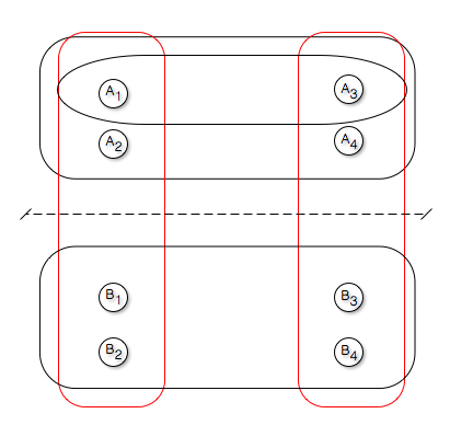
An example of simple 4-way partitioning
Here the hypergraph is partitioned into two parts with vertices \(A_i\) is one part and \(B_i\) in another. Two hyperedges are cut (highlighted in red).
What is it for?
Probably the most important application of hypergraph partitioning is VLSI design. Within the integrated chip, logic often has to be partitioned into clusters, subject to area size and I/O bounds. The hypergraph is a natural representation of the circuit netlist connections: vertices correspond to modules and hyperedges correspond to signal nets, such that each hyperedge contains the vertices (modules) that the net connects.
VLSI design is also the field where a second hypergraph terminology originates. According to it, hypergraph consists of three sets: hyperedge labels (or nets), vertices and pins2. Each pin connects a vertex to a hyperedge label. In a way, this interprets the hypergraph as a bipartite graph, with vertices in one part, hyperedges in another and a set of edges (pins) connecting the two.
In general, for many problems hypergraph provides a better approximation of the structure of the problem than a graph. One very illustrative example is given in the following figure (taken from “Graph partitioning” by Bichot et al.):
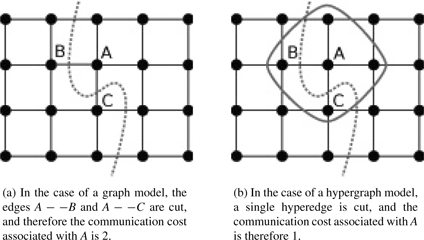
Here we’re trying to bisect a grid, in which each vertex requires information of the neighboring vertices. In graph approximation, the number of required inter-partition communications is equal to two. But a single communication between partitions is sufficient to provide information about A to B and C (since both B and C are in the same part).
Therefore in this problem hypergraph provides an accurate model, whereas graph is only an approximation.
Another important application is partitioning of sparse matrices. This is often done in order to improve matrix-vector product efficiency (SpMV) by decreasing communication volumes and spreading non-zeros evenly over the processors.
A hypergraph can be constructed from a matrix \(A\) in the following way: each row is a hyperedge, each column is a vertex and a vertex \(i\) belongs to hyperedge \(j\) if there is a non-zero element at the intersection of \(i^{th}\) row and \(j^{th}\) column (i.e. if \(A_{ij}\neq 0\)).
The following figure gives an example of a sparse matrix distributed over four processors 3.
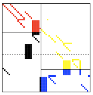
An example of a sparse matrix partitioned into four parts
How does one partition a hypergraph?
By far the most popular approach is multilevel. It is used by all popular hypergraph partitioners (hMetis, PaToH, Zoltan). Multilevel approach, inspired by multigrid computational methods, can be found in every corner of the computationally-intensive part of computer science. It is characterized by a V-cycle, with the left side of the “V” corresponding to iterative coarsening or restricting of the problem, and the right side – to uncoarsening and interpolating the solution.
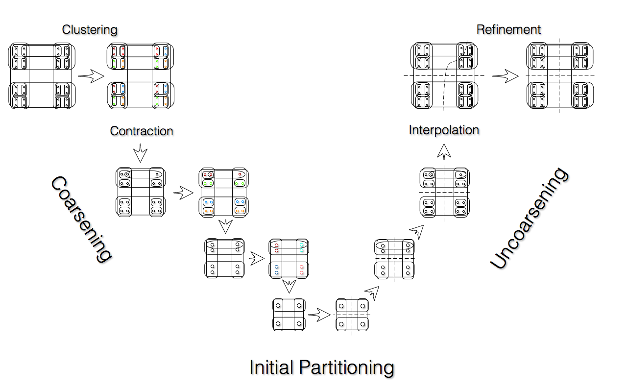
An example of V-cycle for hypergraph partitioning
As shown in the figure, multilevel hypergraph partitioning consists of three stages: coarsening (left side of the “V”), initial partitioning (bottom of the “V”) and refinement (right side of the “V”). In coarsening stage, on each level vertices are usually greedily merged with a neighbor based on the number of the shared hyperedges. Coarsening step is repeated until the hypergraph becomes small enough so that a solution (initial partitioning) can be computed quickly (usually this means coarsening it until it only has ~100 vertices). Then the initial partitioning is refined using a vertex-moving search heuristic, which is almost always a variation on KL-FM.
So what is my research about?
This is where I can finally explain my research! My work focuses around improving the quality of coarsening (left side of the “V”) by improving the quality of matching. That is, I’m working towards making more accurate decisions when choosing which vertices to merge. My first paper (with I. Safro and J. Chen) introduces a new similarity metric for vertices in hypergraph. But that is a story for a different blog post…
- In other words, if graph is a pair of sets \(G=(V,E)\), where \(V\) is the set of vertices, \(E\) is the set of edges and the cardinality of each element in \(E\) is two (\(|e| = 2\,\forall e\in E\)), a hypergraph is the same pair \(H = (V,E)\), except the cardinality of elements in \(E\) is not limited. [return]
- As opposed to just two sets: hyperedges and vertices. [return]
- From “A Two-Dimensional Data Distribution Method for Parallel Sparse Matrix-Vector Multiplication by B. Vastenhouw et al.” [return]